Scientific Audio Processing, Part II - How to make basic Mathematical Signal Processing in Audio files using Ubuntu with Octave 4.0
In the previous tutorial, we saw the simple steps to read, write and playback audio files. We even saw how we can synthesize an audio file from a periodic function such as the cosine function. In this tutorial, we will see how we can do additions to signals, multiplying signals (modulation), and applying some basic mathematical functions to see their effect on the original signal.
Adding Signals
The sum of two signals S1(t) and S2(t) results in a signal R(t) whose value at any instant of time is the sum of the added signal values at that moment. Just like this:
R(t) = S1(t) + S2(t)
We will recreate the sum of two signals in Octave and see the effect graphically. First, we will generate two signals of different frequencies to see the signal resulting from the sum.
Step 1: Creating two signals of different frequencies (ogg files)
>> sig1='cos440.ogg';                  %creating the audio file @440 Hz
>> sig2='cos880.ogg';                  %creating the audio file @880 Hz
>> fs=44100;                           %generating the parameters values (Period, sampling frequency and angular frequency)
>> t=0:1/fs:0.02;
>> w1=2*pi*440*t;
>> w2=2*pi*880*t;
>> audiowrite(sig1,cos(w1),fs);        %writing the function cos(w) on the files created
>> audiowrite(sig2,cos(w2),fs);
Here we will plot both signals.
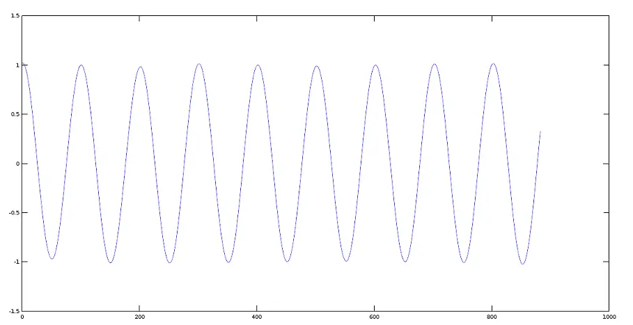
Plot of Signal 1 (440 Hz)
>> [y1, fs] = audioread(sig1);
>> plot(y1)
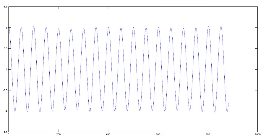
Plot of Signal 2 (880 Hz)
>> [y2, fs] = audioread(sig2);
>> plot(y2)
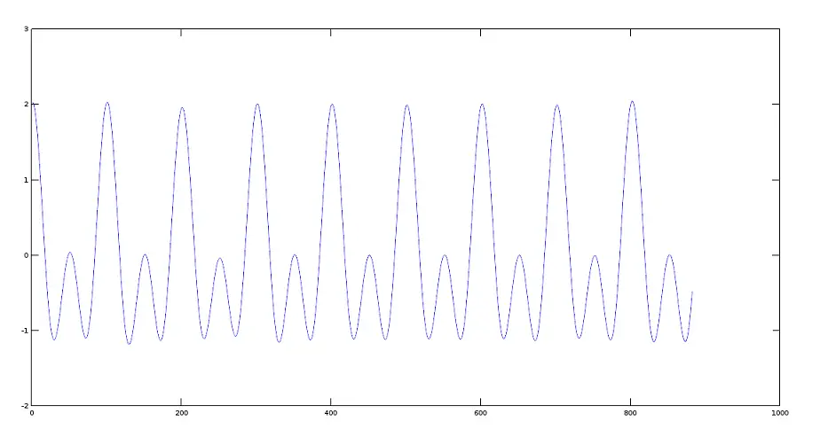
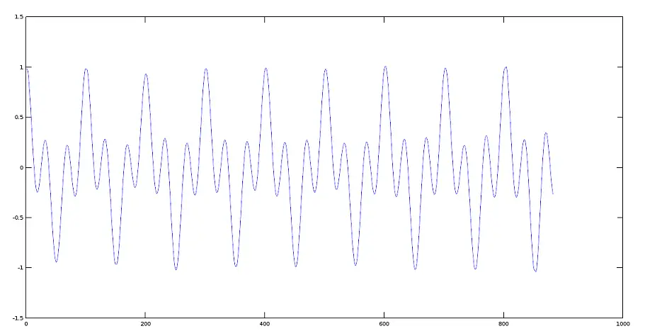
Step 2: Adding two signals
Now we perform the sum of the two signals created in the previous step.
>> sumres=y1+y2;
>> plot(sumres)
Plot of Resulting Signal
The Octaver Effect
In the Octaver, the sound provided by this effect is characteristic because it emulates the note being played by the musician, either in a lower or higher octave (according as it has been programmed), coupled with sound the original note, ie two notes appear identically sounding.
Step 3: Adding two real signals (example with two musical tracks)
For this purpose, we will use two tracks of Gregorian Chants (voice sampling).
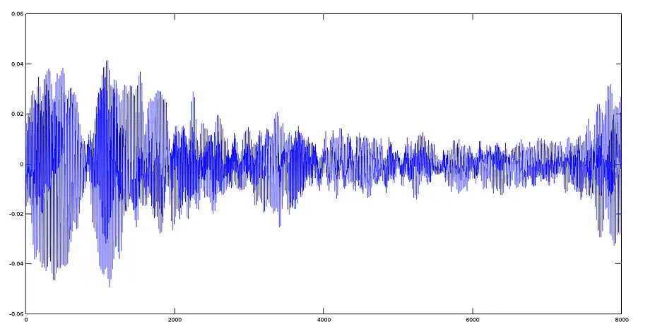
Avemaria Track
First, will read and plot an Avemaria track:
>> [y1,fs]=audioread('avemaria_.ogg');
>> plot(y1)
Hymnus Track
Now, will read and plot an hymnus track
>> [y2,fs]=audioread('hymnus.ogg');
>> plot(y2)
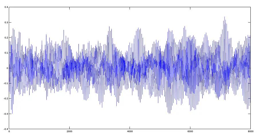
Avemaria + Hymnus Track
>> y='avehymnus.ogg';
>> audiowrite(y, y1+y2, fs);
>> [y, fs]=audioread('avehymnus.ogg');
>> plot(y)
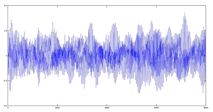
The result, from the point of view of audio, is that both tracks will sound mixed.
Product of two Signals
To multiply two signals, we have to use an analogous way to the sum. Let´s use the same files created previously.
>> sig1='cos440.ogg';                  %creating the audio file @440 Hz
>> sig2='cos880.ogg';                  %creating the audio file @880 Hz
>> product='prod.ogg';                 %creating the audio file for product
>> fs=44100;                           %generating the parameters values (Period, sampling frequency and angular frequency)
>> t=0:1/fs:0.02;
>> w1=2*pi*440*t;
>> w2=2*pi*880*t;
>> audiowrite(sig1, cos(w1), fs);      %writing the function cos(w) on the files created
>> audiowrite(sig2, cos(w2), fs);
>> [y1,fs]=audioread(sig1);
>> [y2,fs]=audioread(sig2);
>> audiowrite(product, y1.*y2, fs);    %performing the product
>> [yprod,fs]=audioread(product);
>> plot(yprod);                        %plotting the product
Note: we have to use the operand '.*' because this product is made, value to value, on the argument files. For more information, please refer to the manual of product operations with matrices of Octave.
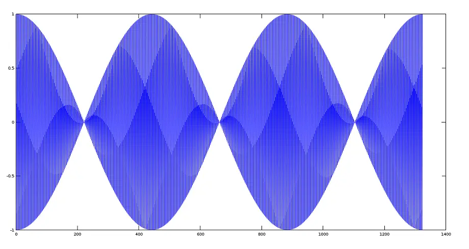
Plot of Resulting Product Signal
Graphical effect of multiplying two signals with a big fundamental frequency difference (Principles of Modulation)
Step 1:
Create an audio frequency signal with a 220Hz frequency.
>> fs=44100;
>> t=0:1/fs:0.03;
>> w=2*pi*220*t;
>> y1=cos(w);
>> plot(y1);
Step 2:
Create a higher frequency modulating signal of 22000 Hz.
>> y2=cos(100*w);
>> plot(y2);
Step 3:
Multiplying and plotting the two signals.
>> plot(y1.*y2);
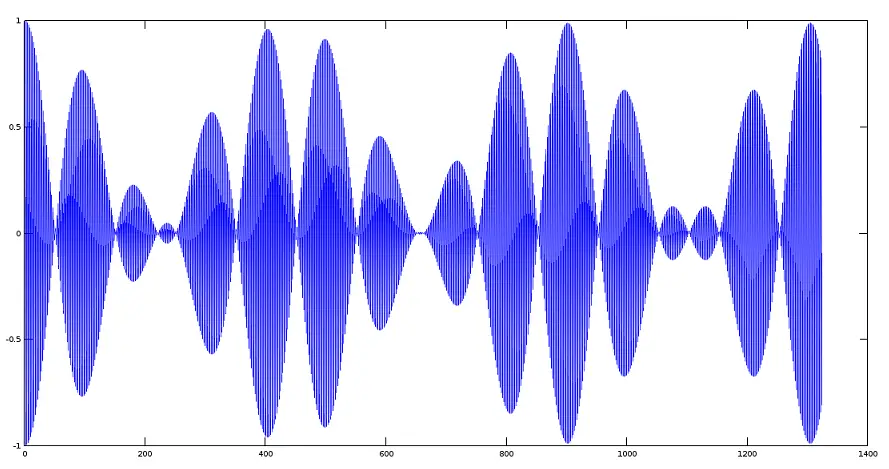
Multiplying a signal by a scalar
The effect of multiplying a function by a scalar is equivalent to modify their scope and, in some cases, the sign of the phase. Given a scalar K, the product of a function F(t) by the scalar is defined as:
>> [y,fs]=audioread('cos440.ogg');        %creating the work files
>> res1='coslow.ogg';
>> res2='coshigh.ogg';
>> res3='cosinverted.ogg';
>> K1=0.2;                                %values of the scalars
>> K2=0.5;
>> K3=-1;
>> audiowrite(res1, K1*y, fs);            %product function-scalar
>> audiowrite(res2, K2*y, fs);
>> audiowrite(res3, K3*y, fs);
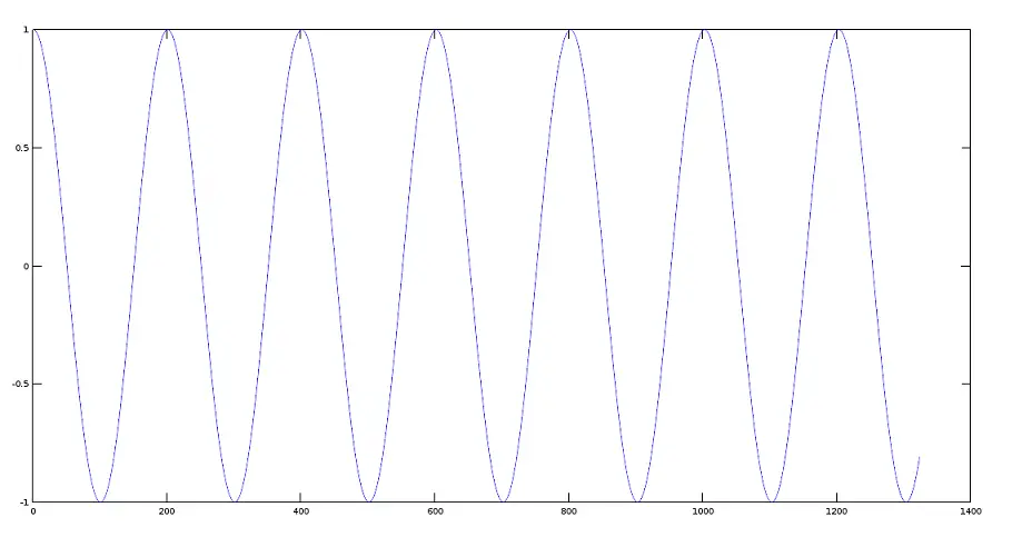
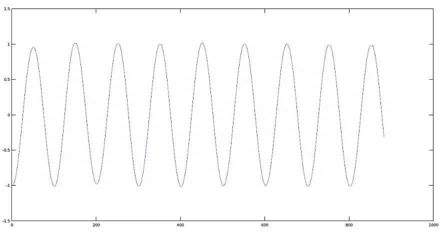
Plot of the Original Signal
>> plot(y)
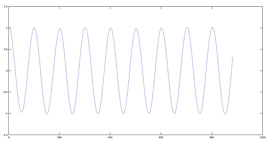
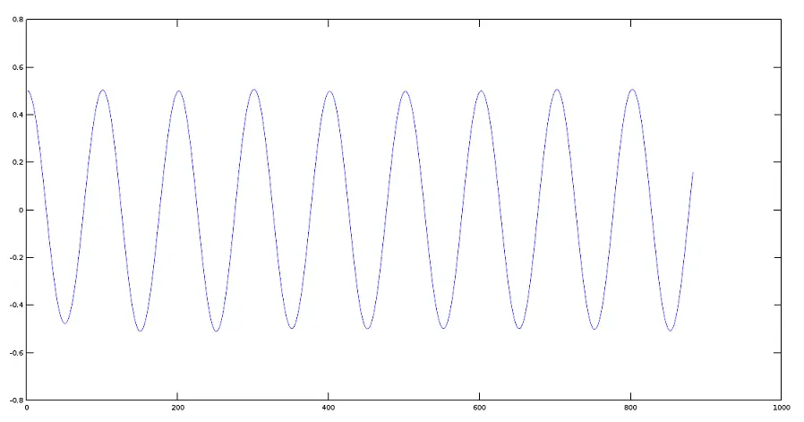
Plot of a Signal reduced in amplitude by 0.2
>> plot(res1)
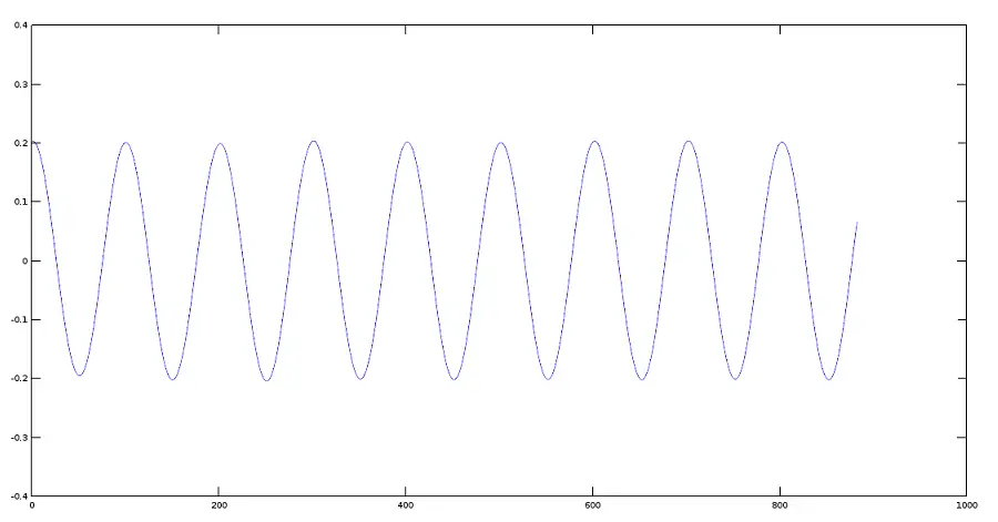
Plot of a Signal reduced in amplitude by 0.5
>> plot(res2)
Plot of a Signal with inverted phase
>> plot(res3)
Conclusion
The basic mathematical operations, such as algebraic sum, product, and product of a function by a scalar are the backbone of more advanced operations among which are, spectrum analysis, modulation in amplitude, angular modulation, etc. In the next tutorial, we will see how to make such operations and their effects on audio signals.

