Get Started With GNUPlot

GNUPlot is an actively developed freely distributed non-open source command line graphing and plotting software tool that was initially released back in 1986. GNUPlot can be useful for a wide spectrum of applications, so here comes a quick guide that will help you understand how it works, get to play with its basic functionality, and learn how to take your first steps with it the easy way.

Command Line

To run GNUPlot, you simply open a terminal, type “gnuplot” and hit enter. This will launch the software tool so you are ready to set your variables and start plotting. For example, in the following screenshot, I have set the “y” variable to have a value of “5” and then plotted the corresponding graph by typing “plot (y)” and hitting enter as shown below.

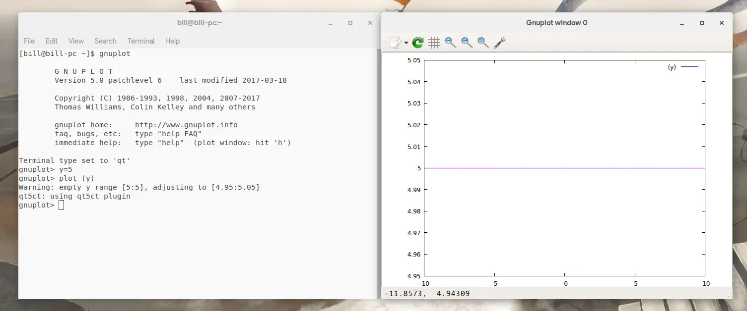
Note that GNUPlot warns me that I have not defined a value range for my graph so it has automatically assigned one for me. If I want to do this myself, I can define a specific range by adding two numbers separated by a colon inside square brackets as shown in the following screenshot.

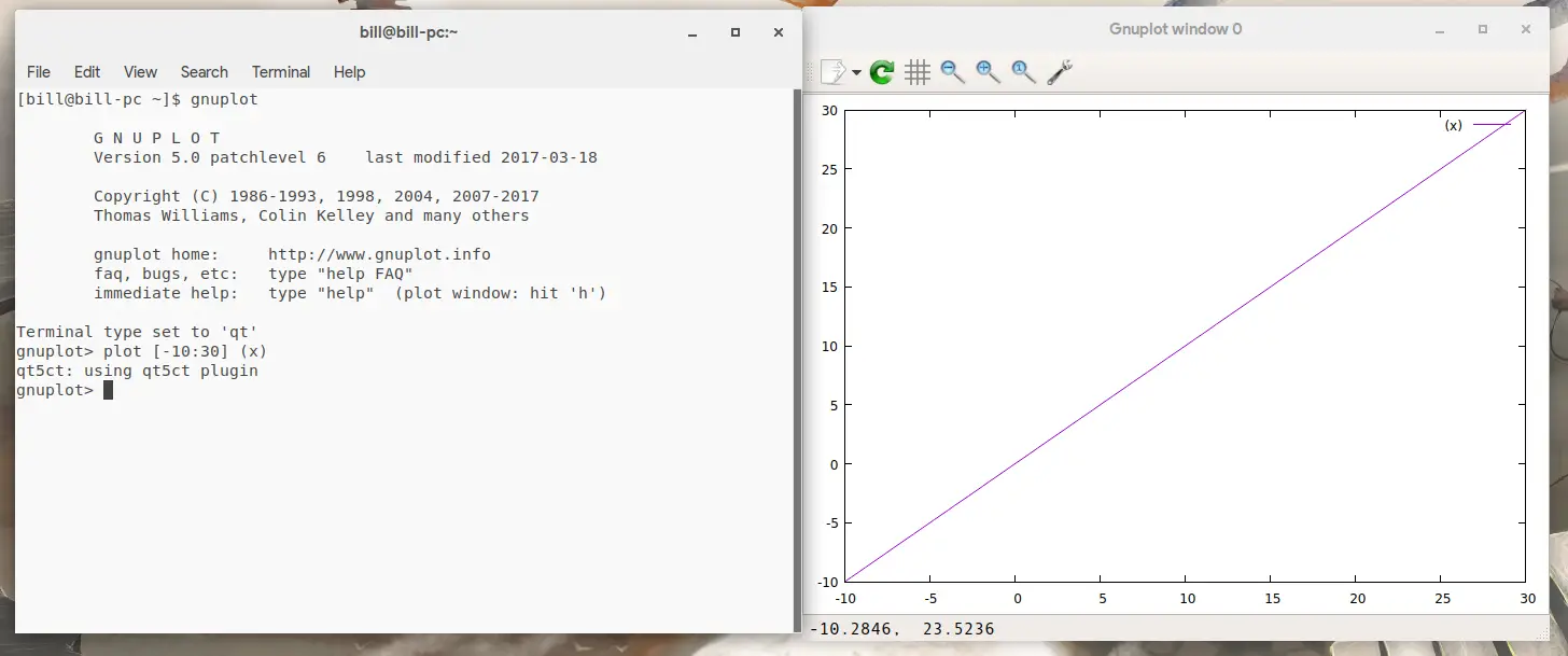
GNUPlot supports all the functions of the Unix mathematic library with most of them supporting integer, real, and complex arguments. You may plot different functions by simply separating them with a comma and the software will assign them with an individual line color given in the legend. Here is an example of three functions in a range of 80 units using the sine, inverse tangent (tan^-1x), and the cosine of the inverse tangent.

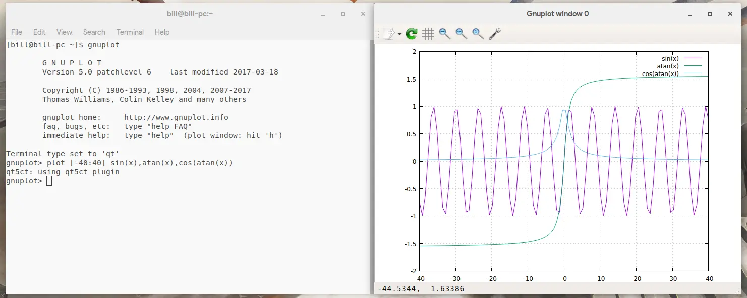
While you can do anything and harvest the full power of GNUPlot from the command line, I will continue to an example of a graphical interface to keep things easier and simpler for the most.

Graphical

My favorite option is the Qt-based “Cueplot” which has been around for quite a while and works well enough. Resuming from where I stopped in the command line, I will showcase how to change the colors and thickness of the graph lines on Cueplot, how to export them, and then proceed further by plotting 3D and surface graphs.

In the Cueplot, you may add functions from the box on the top, then activate the entry by checking the box on the right and clicking on either 2D plot or 3D plot for the generation of the corresponding graph.

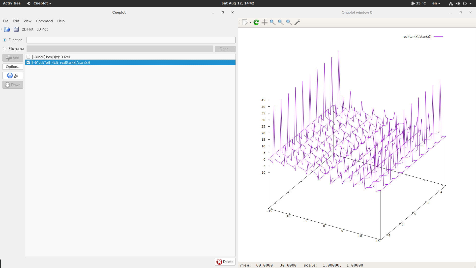
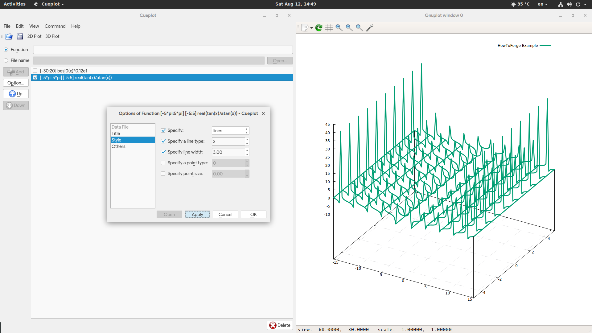
Now to change the thickness and color of the lines, as well as to change their color and the title, you may select the function and then click on the “Options” button on the left. This will open up a new window with options where you can add a new name for the legend, and then select the style options to change the color through the “specify a line type” and also the width. For the changes to apply, you will need to press the “3D Plot” once again.

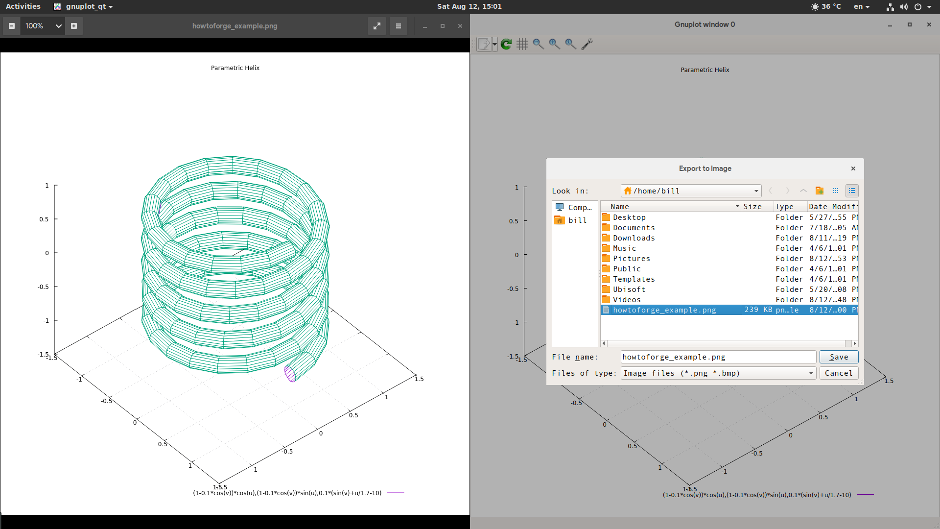
The easiest way to save that graph now is to export it in the form of a png image, which you can easily do by clicking on the export button located on the top left of the graph window and selecting the “Export to Image” option (although the other options are useful as well).

Resources

This concludes the basic scope of this quick guide as you should be able to start playing with functions now on GNUplot, further exploring its possibilities. To help you with that, here is a website containing various examples of functions that I used in this tutorial: http://gnuplot.sourceforge.net/demo/, and also here is a cheat sheet containing the functions that you can use on the software: http://www.gnuplot.info/docs_4.0/gpcard.pdf.