

I recently decided to revisit Football-o-Genetics, an application I developed in 2013 that attempts to "evolve" near-optimal football offensive play calling strategies. The application uses play-by-play data and ideas from both artificial intelligence (specifically, genetic algorithms) and advanced statistics (in the form of a Markov model of an offensive drive) to achieve its goal. I developed Football-o-Genetics shortly after dropping out of a PhD program in evolutionary biology, so it's probably not all that surprising that I chose genetic algorithms (which I first encountered in Russell and Norvig's classic Artificial Intelligence textbook) as my optimization algorithm of choice.
Almost four years later, my understanding of all things AI is much broader and deeper than it was at that time, and it's clear to me now that other reinforcement learning approaches are better suited for this particular problem. I thought it would be fun to give one of these other reinforcement learning approaches a shot. Specifically, I chose to go with Q-learning, which is a technique for learning "optimal action-selection [policies]"; i.e., it can tell you the best action to take in different situations when you're trying to maximize some reward. Q-learning is an extremely flexible and powerful technique, and it was a key component in Google's AI that learned to play Atari at superhuman levels.
The Q-learning algorithm is actually surprisingly simple to implement; all it requires is some representation of the state (i.e., situation), a list of available actions, and a reward signal. For the play-calling problem, I chose to represent each state using three components: the field position, the down, and a discretized representation of the distance (i.e., "Short," "Medium," or "Long") to a first down. For example, if a team was on its own 33-yard line and it was second down and 10 yards to go, the state was encoded as "33-2nd-Long." This encoding corresponds to approximately 100 × 3 × 3 = 900 states (there are actually fewer states because of the way I handled first down and goal situations). (See below for why I chose to discretize the distance.)
The actions available to the algorithm correspond to different play/player combinations. The two plays are "Rush" or "Pass," and each play is combined with one of several players (running backs for rushes and quarterbacks for passes). That means there are approximately #RBs + #QBs = #actions to choose from for any given state.
At this point, the algorithm is ready to be trained. Training consists of simulating offensive drives (each drive is an "episode" in the reinforcement learning vernacular) and updating the Q values accordingly. An offensive drive begins by randomly generating a starting field position. The algorithm then selects an action using an ϵ-greedy strategy. When an action is selected, the number of yards gained on the play is sampled from actual data for that particular play/player combination from the season. This is why I chose to discretize the distance; it makes it easy to approximate the true distribution of yards gained for a particular play/player combination. To be more explicit, a given down/distance/play/player combination is associated with a list, e.g., down_and_distance["2ndMedPass"]["C Newton"] = [-2, 1, 4, 0, 0, 0, 17, 13, 11, 0, 0, 17, 0, 0, 0, 0, 3, 27, 4, 4, 5, 0, 0, -2, 0, 0, 3, 11, 1] and the yards gained on a play are randomly drawn from that list. The data used to train the model is from 2012 because that's the data I had collected for the original application.
The simulation then proceeds like a typical football game with the down and distance updated accordingly. Turnovers are generated with probabilities estimated from actual turnover data from the season. When a turnover occurs or the drive reaches fourth down, the episode is terminated and the simulation restarts from the beginning. All play outcomes have a reward signal of zero except for touchdowns, which have a reward signal of one.
opensource.com
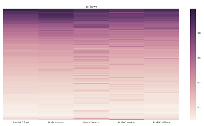
As you can see in Figure 1, the closer you get to the end zone (the top of the plot), the more likely it is that the drive will eventually result in touchdown. You can also see that, in general, allowing Cam Newton to either run or pass was generally the best strategy for the Panthers on first down in 2012.
While these results are interesting, they don't actually represent an optimal play-calling strategy, because the model treats the defense as if it were part of the environment rather than an adversary capable of adapting to the offense's tendencies. Unfortunately, defensive play calling data is hard to come by, but I've decided to outline how I would approach the problem if I had the time to sit down and watch a bunch of football games. (A man can dream, can't he?)
Offensive plays have a nice, natural categorization—rushes and passes—but categorizing defensive plays isn't quite as easy. While there are some informative descriptors of defensive plays available, like "blitz" or "zone" vs. "man," none of them seem to capture the full essence of the defensive play. With that being the case, I propose that number of rushed defenders fills that role. While you don't get precise information regarding the defense's coverage with this categorization, it does give you a sense of the defense's "aggressiveness" on the play, and I suspect that property will translate to useful statistical properties. For example, I would expect there to be a negative relationship between the number of rushed defenders and the average yards gained by the offense on a rush play.
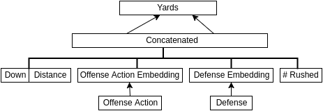
So, having established a categorization for defensive play calls, the next step is to decide how yardage would be generated given an offensive play call and a defensive play call. I think I would take an approach similar to what I did with (batter|pitcher)2vec, where I built a model that learns distributed representations of batters and pitchers by attempting to predict the outcome of every pitch (e.g., strike, ball, fly out to left field) over several baseball seasons. The analogous football model, which I shall dub (offense|defense)2vec, might look something like Figure 2.
opensource.com
The inputs to this model would be the down, distance, offensive action (e.g., "Pass-C Newton"), defensive team, and number of defenders rushed on the play. The number of offensive actions is approximately equal to #teams × (#QBs + #RBs), which we'll guesstimate is around 32 × (1.5 + 2.5) = 128. In the case of the output, performing a regression might seem like the obvious choice, but optimizing a regression model using mean squared error is equivalent to assuming a Gaussian distribution on the output (conditioned on the model and input) from a probabilistic perspective, and I don't think a Gaussian is appropriate here. On the other hand, treating all of the possible yardage gains (i.e., from -99 to 99) as distinct classes is probably needlessly granular and may make learning noisy.
opensource.com
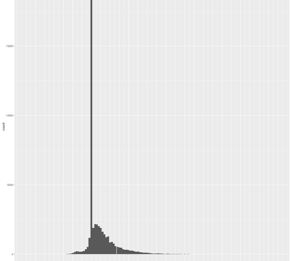
Looking at the histogram in Figure 3 (generated from the 2015 NFL dataset released by Carnegie Mellon University), I think a reasonable output layer might have one bin for 100 to 40.5 yards (which represents 1% of the distribution), one bin for zero yards, bins for -15 to -5.5 yards and -5.5 to -0.5 yards, and a bin for each two-yard span beginning at 0.5 (so 0.5 to 2.5 would be the first bin) and ending at 40.5 (so the last bin is 38.5 to 40.5).
To generate yards for a given play, you would first sample one of the bins using the probability distribution provided by the down, distance, offensive action, defense, and number of rushed defenders. From there, you would uniformly sample from the yards contained in the bin. So, for the bin ranging from 18.5 to 20.5 yards, you would have a 50% chance of gaining 19 yards and a 50% chance of gaining 20 yards. There are obviously more complicated things you could do with these distributions, but the binned approach seems like a reasonable, simple approximation. At this point, the only thing left to do would be to implement minimax Q-learning, then re-run the simulations using the new yardage generator.
Anyway, that's all for the hypotheticals. You can download the Football-o-Genetics source code on GitHub. If you've done similar work, or if this project ends up inspiring you to work on something of your own, I'd love to hear about it.
Reprinted with permission from Red Hat senior software engineer Michael A. Alcorn's blog.


4 Comments