How to install and use profiling tool Gprof on Linux
On this page
There's no doubt that testing is an integral and one of the most important aspects of the software development process. And by testing, we don't mean just testing the code for bugs - of course, bug detection is important as nobody would want their software to be buggy - performance of the code also equally matters these days.
If broken down to the last bit, performance testing effectively tests how much time a particular piece of code - say a function - is consuming. As is usually the case, a function or a group of functions may correspond to one of the many features of a software. So, if through performance testing, we can enhance the performance of these functions in code, the overall performance of the software becomes better.
If you are a programmer, who writes code in C, Pascal, or Fortran77 programming language and uses Linux as the development platform, you'll be glad to know that there exists a powerful tool through which you can check the performance of your code - the tool in question is Gprof. In this tutorial, we'll be discussing the details of how you can download, install, and use this tool.
Before we move ahead, please note that all the examples and instructions mentioned in this tutorial have been tested on Ubuntu 14.04LTS and the Gprof version used is 2.24.
What is Gprof?
So, what exactly is Gprof? According to the tool's official documentation, it gives users an execution profile of their C, Pascal, or Fortran77 programs. What Gprof basically does is, it calculates the amount of time spent in each routine or function. "Next, these times are propagated along the edges of the call graph. Cycles are discovered, and calls into a cycle are made to share the time of the cycle."
If all this sounds a bit confusing at this point (especially the part in quotes), don't worry, as we'll make things clear through an example. So, read on.
Download and Install Gprof
First check whether or not the tool is already installed on your system. To do this, just run the following command in a terminal.
$ gprof
If you get an error like:
$ a.out: No such file or directory
then this would mean that the tool is already installed. Else you can install it using the following command:
$ apt-get install binutils
Gprof Usage
Needless to say, the best way to understand a tool like Gprof is through a practical example. So, we'll start off with a C language program, which we'll be profiling through Gprof. Here's the program:
//test_gprof.c

#include<stdio.h>

void func4(void)
{
    printf("\n Inside func4() \n");
    for(int count=0;count<=0XFFFF;count++);
}

void func3(void)
{
    printf("\n Inside func3() \n");
    for(int count=0;count<=0XFFFFFFF;count++);
}

void func2(void)
{
    printf("\n Inside func2() \n");

    for(int count=0;count<=0XFFF;count++);

    func3();
}

void func1(void)
{
    printf("\n Inside func1() \n");
    for(int count=0;count<=0XFFFFFF;count++);

    func2();
}

int main(void)
{
    printf("\n main() starts...\n");
    for(int count=0;count<=0XFFFFF;count++);

    func1();
    func4();
    printf("\n main() ends...\n");

    return 0;
}
Please note that the code shown above (test_gprof.c) is specifically written to explain Gprof - it's not taken from any real-life project.
Now, moving on, the next step is to compile this code using gcc. Note that ideally I would have compiled the above code using the following command:
$ gcc -Wall -std=c99 test_gprof.c -o test_gprof
But since we've to profile the code using Gprof, I'll have to use the -pg command line option provided by the gcc compiler. So, the command becomes:
$ gcc -Wall -std=c99 -pg test_gprof.c -o test_gprof
If you take a look at gcc's man page, here's what it says about the -pg option:
"Generate extra code to write profile information suitable for the analysis program gprof. You must use this option when compiling the source files you want data about, and you must also use it when linking."
Now, coming back to the above command, after it's executed successfully, it will produce a binary named test_gprof in the output. The next step is to launch that executable. Here's how I launched the binary in my case:
$ ./test_gprof
Once the command is executed, you'll see that a file named gmon.out will be generated in the current working directory.
$ ls gmon*
gmon.out
It is this file which contains all the information that the Gprof tool requires to produce a human-readable profiling data. So, now use the Gprof tool in the following way:
$ gprof test_gprof gmon.out > profile-data.txt
Basically, the generic syntax of this command is:
$ gprof [executable-name] gmon.out > [name-of-file-that-will-contain-profiling-data]
Now, before we see the information the profile-data.txt file contains, it's worth mentioning that that the human-readable output Gprof produces is divided into two parts: flat profile and call graph. Here's what the man page of Gprof says about information under these two sections:
"The flat profile shows how much time your program spent in each function, and how many times that function was called. If you simply want to know which functions burn most of the cycles, it is stated concisely here."
"The call graph shows, for each function, which functions called it, which other functions it called, and how many times. There is also an estimate of how much time was spent in the subroutines of each function. This can suggest places where you might try to eliminate function calls that use a lot of time."
Armed with this information, now you'll be in a better position to understand the data present in your profiling output file (profile-data.txt in my case). Here's the flat profile in my case:
Flat profile:

Each sample counts as 0.01 seconds.
 %    cumulative self           self    total
 time seconds    seconds calls  ms/call ms/call  name
 96.43 0.81      0.81      1    810.00  810.00   func3
 3.57 0.84       0.03      1    30.00   840.00   func1
 0.00 0.84       0.00      1    0.00    810.00   func2
 0.00 0.84       0.00      1    0.00    0.00     func4
And here's what each field means:
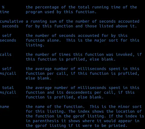
Moving on, here's the call graph in my case:
Call graph (explanation follows)


granularity: each sample hit covers 4 byte(s) for 1.19% of 0.84 seconds

index % time self children called name
             0.03 0.81     1/1       main [2]
[1]    100.0 0.03 0.81      1     func1 [1]
             0.00 0.81     1/1       func2 [3]
-----------------------------------------------
                                     <spontaneous>
[2]    100.0 0.00 0.84            main [2]
             0.03 0.81     1/1       func1 [1]
             0.00 0.00     1/1       func4 [5]
-----------------------------------------------
             0.00 0.81     1/1       func1 [1]
[3]    96.4  0.00 0.81      1     func2 [3]
             0.81 0.00     1/1       func3 [4]
-----------------------------------------------
             0.81 0.00     1/1       func2 [3]
[4]    96.4  0.81 0.00      1      func3 [4]
-----------------------------------------------
             0.00 0.00     1/1       main [2]
[5]    0.0   0.00 0.00      1      func4 [5]
The following screenshots explain the information call graph contains:
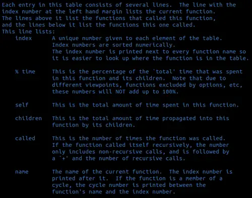
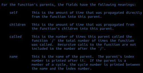
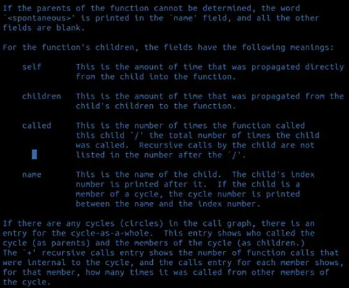
If you're wondering about the source of above screenshots, let me tell you that all this information is there in the output file that contains the profiling information, including flat profile and call graph. In case you want this information to be omitted from the output, you can use the -b option provided by Gprof.
Conclusion
Needless to say, we've just scratched the surface here, as Gprof offers a lot of features (just take a look at its man page). However, whatever we've covered here should be enough to get you started. In case you already use Gprof, and want to share something related to the tool with everyone here, just drop in a comment below.

